Financial concepts

Keldan has gathered the main concepts used in the financial sector, with a few worked examples of how they are applied.

Financial management
Interest
Time value of money
Risk and return
Bonds
The annual accounts
Financial ratios
Cost of capital
Company valuation

Financial management

The value of a company is the key quantity in all financial management, and it is determined chiefly by three things: (1) the size of the free cash flow (FCF) the company generates, together with (2) its timing and (3) the risk attached to that cash flow.

All else being equal, risk and the cost of capital move together; risk and return are covered in more detail in part 4. The weighted average cost of capital (WACC) is the average required return that all investors demand of a company. The value of a company can be described with the following equation:

1.1

Value =

\frac{FCF_1}{(1 +WACC)^1} + \frac{FCF_2}{(1 + WACC)^2} + \cdots + \frac{FCF_{\infty}}{(1 + WACC)^\infty}

Free cash flow (FCF) is covered in more detail in part 6, the weighted average cost of capital (WACC) in part 8, and company valuation in part 9.

Interest

Interest is the fee a borrower pays for the use of capital over a given period, which makes it a time-related cost. In almost all cases interest is quoted on an annual basis and as a percentage of the principal of the loan. Interest comes in two forms: (1) simple interest and (2) compound interest, the difference being whether interest is calculated on previously accrued interest or not.

Simple interest

When interest is calculated on the principal alone, it is called simple interest.

2.1

Interest payment =

P \cdot i \cdot n

2.2

Principal at end of period =

S = P + (P \cdot i \cdot n)

P = principal at start of period
i = nominal interest rate
n = time (in years)

Example 2-1

Gunnar buys a bond with a face value of ISK 100,000 carrying 6% nominal interest, maturing in six months. What will the interest payment be, and how much does he get back?

Solution

Compound interest

When interest is calculated on the principal together with previously accrued interest, it is called compound interest.

2.3

Interest payment =

P \cdot ((1+i)^n - 1)

2.4

Principal at end of period =

S = P \cdot (1 + i)^n

P = principal at start of period
i = nominal interest rate
n = time (in years)

Example 2-2

Jón buys a bond with a face value of ISK 100,000 carrying 6% nominal interest, maturing in three years. What will the interest payment be, and how much does he get back?

Solution

The example with Jón assumes that the 6% nominal interest compounds annually, which is the convention unless stated otherwise. But since compound interest accrues on both the principal and previously accrued interest, how often it is calculated within each period matters a great deal. Compound interest therefore falls into three types: (1) annual compounding, as in example 2–2 above, (2) periodic compounding, and (3) continuous compounding.

Periodic compounding

When compound interest is calculated more than once a year, it is called periodic compounding. The number of compounding periods says how often interest is calculated per year.

2.5

Interest payment =

P \cdot ( ( 1 + \frac{i}{m})^{n \cdot m } - 1 )

2.6

Principal at end of period =

S = P \cdot ( 1 + \frac{i}{m})^{n \cdot m}

P = principal at start of period
i = nominal interest rate
n = time (in years)
m = number of compounding periods per year

Example 2-3

Einar deposits ISK 100,000 in a savings account paying 4% nominal interest, compounded semi-annually. How much interest does Einar earn after one year, and what is the balance?

Solution

Continuous compounding

Had the 4% nominal interest on Einar's account compounded annually, he would only have earned 100,000 · ((1+0.04) – 1) = ISK 4,000 in interest by the end of the year. He therefore gets ISK 40 extra because the interest compounds semi-annually, that is twice a year. Had it compounded quarterly, four times a year, he would have got ISK 60 extra, and had it compounded monthly, twelve times a year, he would have got ISK 74 extra. It is tempting to conclude from this that the more often interest is compounded in a year, the larger the interest payment becomes. The mathematician Leonhard Euler made the remarkable discovery that this is not so. He showed that $\lim\limits_{m \to \infty} (1+\frac{i}{m})^m = e \approx 2{.}71828$ , and today this important number is generally called Euler's number. Euler's discovery shows us that if the nominal interest on Einar's account had compounded infinitely often per year, that is compounded continuously, he would have got ISK 81 extra. This is set out more fully in example 2–4. Interest of this kind is called continuously compounded interest, and Euler's number is used to calculate it.

2.7

Interest payment =

P \cdot (e^{i\cdot n} - 1)

2.8

Principal at end of period =

S = P \cdot e^{i\cdot n}

P = principal at start of period
i = nominal interest rate
n = time (in years)
e = 2.71828...

Example 2-4

Magnús deposits ISK 100,000 in a savings account paying 4% nominal interest, compounded continuously. How much interest does Magnús earn after one year, and what is the balance?

Solution

Effective annual rate

Magnús clearly gets better terms from his bank than Einar does, yet both receive 4% nominal interest. To compare investments with different numbers of compounding periods, their nominal rates are restated as though they were compounded annually. The restated rate is called the effective annual rate. To convert periodic rates into an effective annual rate, use the following equation:

2.9

Effective annual rate =

(1 + \frac{i}{m})^m - 1

i = nominal interest rate
m = number of compounding periods per year

To convert continuously compounded interest into an effective annual rate:

2.10

Effective annual rate =

e^i - 1

i = nominal interest rate

Example 2-5

Compare the effective annual rate available to Einar in example 2–3 with the one available to Magnús in example 2–4.

Solution

In Microsoft ® Excel

The EFFECT function returns the effective annual rate given a nominal rate and a number of compounding periods. The NOMINAL function returns the nominal rate given an effective annual rate and a number of compounding periods.

Real interest rate

The nominal interest rate means interest calculated without regard to the price level, whereas the real interest rate means interest in excess of the change in prices over the same period. The real rate is therefore positive when the nominal rate is higher than inflation over a given period. The real rate can be derived from Fisher's equation as follows:

2.11

Real interest rate =

\frac{1+i}{1+\pi} - 1

i = nominal interest rate
π = inflation

Market interest rates

The market interest rate on any debt security is built up from the real rate on government securities plus the various kinds of risk premium.

2.12

Market interest rate =

r = r^* + IP + DRP + LP + MRP = r_{RF} + DRP + LP + MRP

r^* = real risk-free rate of interest
IP = inflation premium
r^* + IP = r_RF = quoted risk-free rate of interest on treasury bills

DRP = default risk premium
LP = liquidity/marketability premium
MRP = maturity risk premium

Time value of money

The value of any investment rests so heavily on the timing of its cash flows that few areas of finance matter more than the time value of money.

The timeline

The most important aid in time-value-of-money calculations is the timeline.

Time 0 here means today. Time 1 means the point one period from now (or the end of period 1). Time 2 means two periods from now, and time 3 three periods from now. Interest over periods 1 to 3 is taken to be 5%. Present value (PV) always sits at time 0, whereas future value (FV) can sit at the end of any period and is often written FVn, where n is the period in question.

Future value

Compounding is the operation of calculating a future value (FV_n) from a given present value (PV) and a given interest rate. The future value (FV_n) of a single payment is:

3.1

FV_n = PV \cdot (1+i)^n

FV_n = future value at period n
PV = present value
i = interest rate
n = number of periods

Example 3-1

Gunnar plans to invest ISK 100,000 for two years. He requires a 5% return per year. How much does he have after two years?

Solution

Present value

Discounting is the operation of calculating a present value (PV) from a given future value (FV_n) and a given opportunity cost rate, which is the rate on the best available alternative investment carrying the same risk. The present value (PV) of a single payment is:

3.2

PV = \frac{FV_n}{(1+i)^n}

FV_n = future value at period n
PV = present value
i = opportunity cost rate
n = number of periods

Example 3-2

Magnús has to pay ISK 100,000 in two and a half years. If the market rate over that period is 5%, how much does he need to set aside today to cover the payment?

Solution

Annuities

An annuity is a series of equal payments made at regular intervals over a given period. An ordinary annuity pays at the end of each period, whereas an annuity due pays at the start of each period. A perpetuity is a stream of equal payments expected to continue forever.

Future value of an annuity:

3.3

FVA_n = PMT \cdot \displaystyle\sum_{t=1}^n (1 + i)^{n-t} = PMT \cdot (\frac{(1+i)^n - 1}{i})

FVA_n = future value of an annuity over n periods
PMT = the periodic payment
i = interest rate
n = number of periods

Present value of an annuity:

3.4

PVA_n = PMT \cdot (\frac{1 - (1+i)^{-n}}{i})

PVA_n = present value of an annuity over n periods
PMT = the periodic payment
i = interest rate
n = number of periods

Present value of a perpetuity:

3.5

PVP = \frac{PMT}{i}

PVP = present value of a perpetuity
PMT = the periodic payment
i = interest rate

In Microsoft ® Excel

The quantities used in time-value-of-money calculations can be worked out with the following functions:

NPER (= n) returns the number of periods.
RATE (= i) returns the periodic interest rate.
PV returns the present value of the payments.
PMT returns the periodic payment.
FV returns the future value.

In each of these five functions, the values of the other four can be supplied as arguments.

Risk and return

Harry Markowitz described the relationship between risk and return in his 1952 paper Portfolio Selection, and has since often been called the father of modern portfolio theory (MPT). In it he set out how risk in a portfolio could be seen as volatility of returns, and measured by the standard deviation of the portfolio's return.

Risk in securities

The risk of a single security can be split into two parts: (1) market risk and (2) company-specific risk. Investors can protect themselves against company-specific risk by choosing and investing in a well-diversified portfolio. Portfolio risk (σ_p) therefore falls as the number of well-diversified securities in the portfolio rises, converging on the average risk in the market, that is market risk (σ_M), as shown in figure 4–1.

When a single security is added to a well-diversified portfolio, only that security's market risk affects the portfolio. The market risk of a security can be measured by its beta coefficient (b), which shows how much the price of a security moves relative to the swings in the market as a whole.

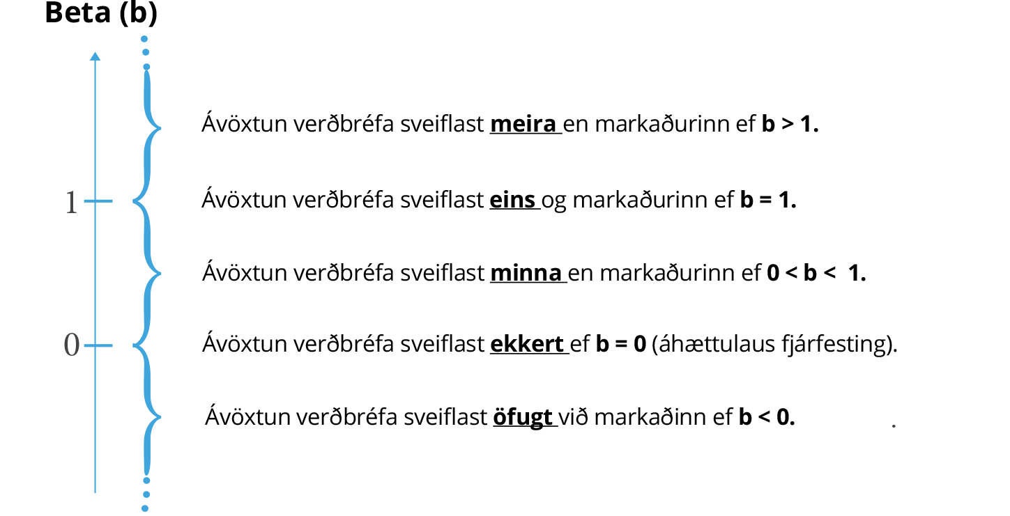
The beta of the market portfolio, which holds every security in the market, is always 1, while the beta of an individual security can be found by simple regression analysis. Beta is defined as the slope coefficient of that regression.

4.1

b_i = (\frac{\sigma_i}{\sigma_M}) \cdot \rho_{iM}

b_i = beta of security i
σ_i = standard deviation of the return on security i
σ_M = standard deviation of the return on the market portfolio
ρ_iM = correlation between the return on security i and the return on the market portfolio

The relationship between risk and return

The best known and most widely used model for describing the relationship between risk and return is the capital asset pricing model (CAPM), which sets out the theoretical relationship between market risk, measured by beta, and required return.

4.2

r_i = r_{RF} + (r_M - r_{RF}) \cdot b_i = r_{RF} + (RP_M) \cdot b_i

r_i = required return on security i
r_M = required return on the market portfolio
r_RF = risk-free rate of return on treasury bills

RP_M = r_M - r_RF = the market risk premium
b_i = beta of security i
(r_M - r_RF) · b_i = risk premium on security i

Example 4-1

The rate on treasury bills is 6% and the market risk premium is 5%. A share has a beta of 0.5. What is the required return on the share?

Solution

From equation 4–2 one can draw the security market line (SML), which describes the required return on security i as a function of the security's beta:

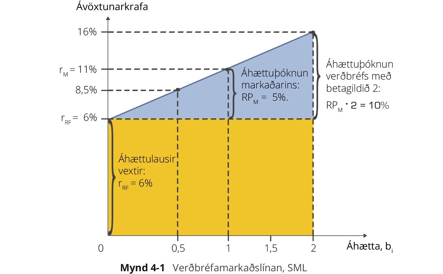
In figure 4–1 the rate on treasury bills is 6% and the market risk premium is 5%, so the required return on the market portfolio is 11%. As in the example above, the required return on the share is 8.5% when beta is 0.5. It can also be seen that the risk premium on a share with a beta of 2 would be 10%, giving a required return of 16%.

Efficient portfolios

A portfolio is said to be efficient if it is composed such that return cannot be increased without also increasing risk, and risk cannot be reduced without also reducing return.

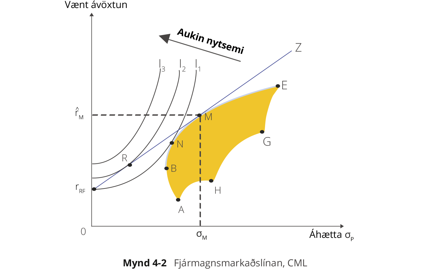
The yellow area in figure 4–2 shows the whole feasible set for securities A, H, G and E. The curve BNME is the efficient frontier, on which every efficient portfolio of those four securities lies. All combinations of risk and return that give an investor with a given risk tolerance the same utility can be described by the indifference curve I_n. If only those four securities were available, the investor would maximise utility by holding portfolio N, known as their optimal portfolio. If the same investor could also buy risk-free treasury bills, which sit at point r_RF, they could increase utility further by buying portfolio R, a blend of portfolio M and treasury bills, moving from indifference curve I₁ to I₂.

The line r_RFMZ is called the capital market line (CML), and it always lies above the efficient frontier except at the tangency point M. It is therefore most efficient for every investor to hold portfolio M and to buy or sell treasury bills according to how much risk they can bear. The capital market line can be described by the following equation:

4.3

r_p = r_{RF} + (\frac{r_M - r_{RF}}{\sigma_M}) \cdot \sigma_p

r_p = expected return on portfolio p
r_M = expected return on the market portfolio
r_RF = risk-free rate of return on treasury bills

σ_p = standard deviation of the return on portfolio p
σ_M = standard deviation of the return on the market portfolio

Fama-French three-factor model

The CAPM described above uses only one variable, beta, to measure the market risk of a security. The model of Eugene Fama and Kenneth French uses three: alongside the market risk premium, it also draws on the company's market capitalisation and its book-to-market ratio (see part 7 on financial ratios).

4.4

r_i = r_{RF} + a_i + (r_M - r_{RF}) \cdot b_i + (r_{SMB}) \cdot c_i + (r_{HML}) \cdot d_i

r_i = required return on security i
r_RF = risk-free rate of return on treasury bills
a_i = alpha of security i

r_M = required return on the market portfolio
r_SMB = return on small-cap companies in excess of large-cap companies
r_HML = return on companies with a high book-to-market ratio in excess of those with a low one

c_i and d_i = coefficients found by simple regression analysis

Other pricing models

The economist Steven Ross at MIT developed a model called Arbitrage Pricing Theory, which uses as many variables to measure risk as the situation requires. Work in behavioural finance takes a different route, pricing securities from psychological analysis of the irrational but predictable ways investors behave in various circumstances.

Bonds

Bonds are the most important class of security anywhere in the world: a country's market interest rates are shaped by trading in them, according to the laws of supply and demand. Bonds, like other securities, are first sold on the primary market, and because they are transferable they are bought and sold on the secondary market once issued.

Types of bond

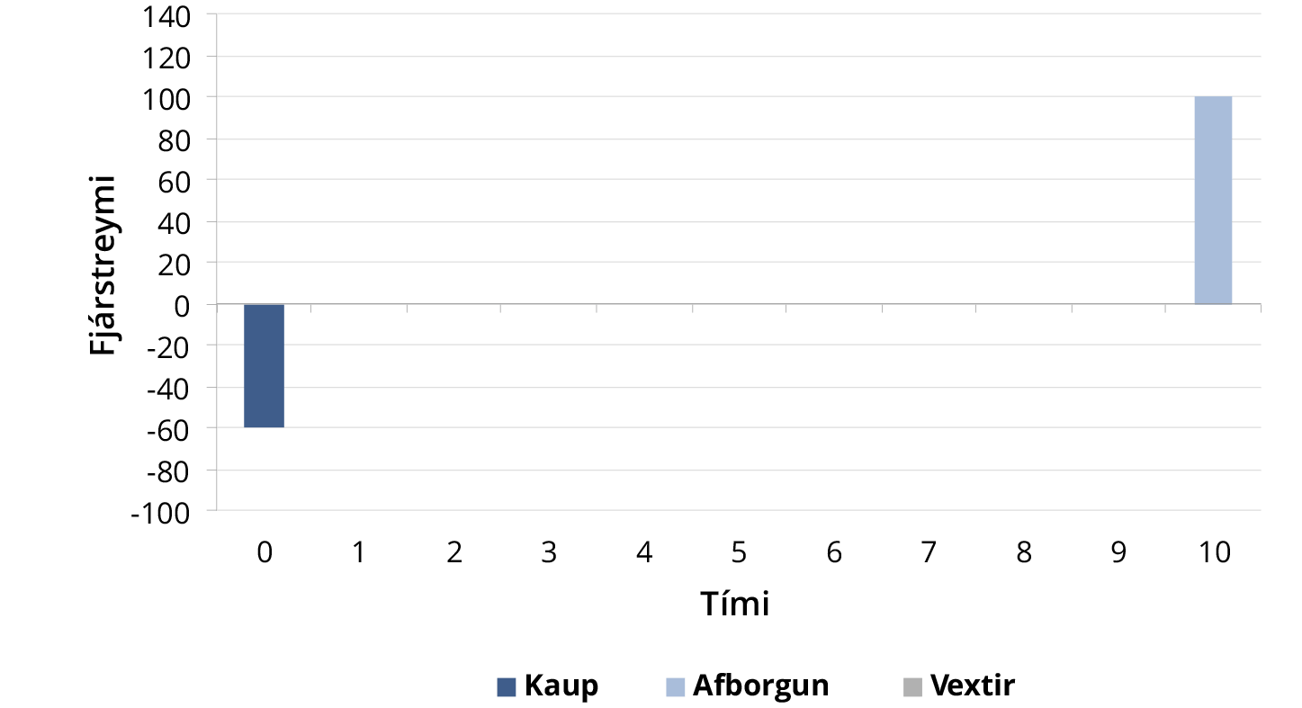
Zero-coupon bond

Carries no nominal interest. Repaid in a single payment of principal at the end of the term.

Example: A 10-year zero-coupon bond sold at a price of 60.

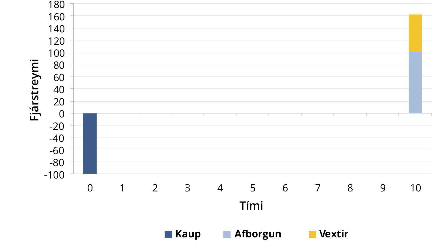
Bullet bond

Carries nominal interest that is added to the principal at regular intervals. Repaid in a single payment of the original principal, interest and compounded interest.

Example: A 10-year bullet bond with 5% nominal interest sold at par.

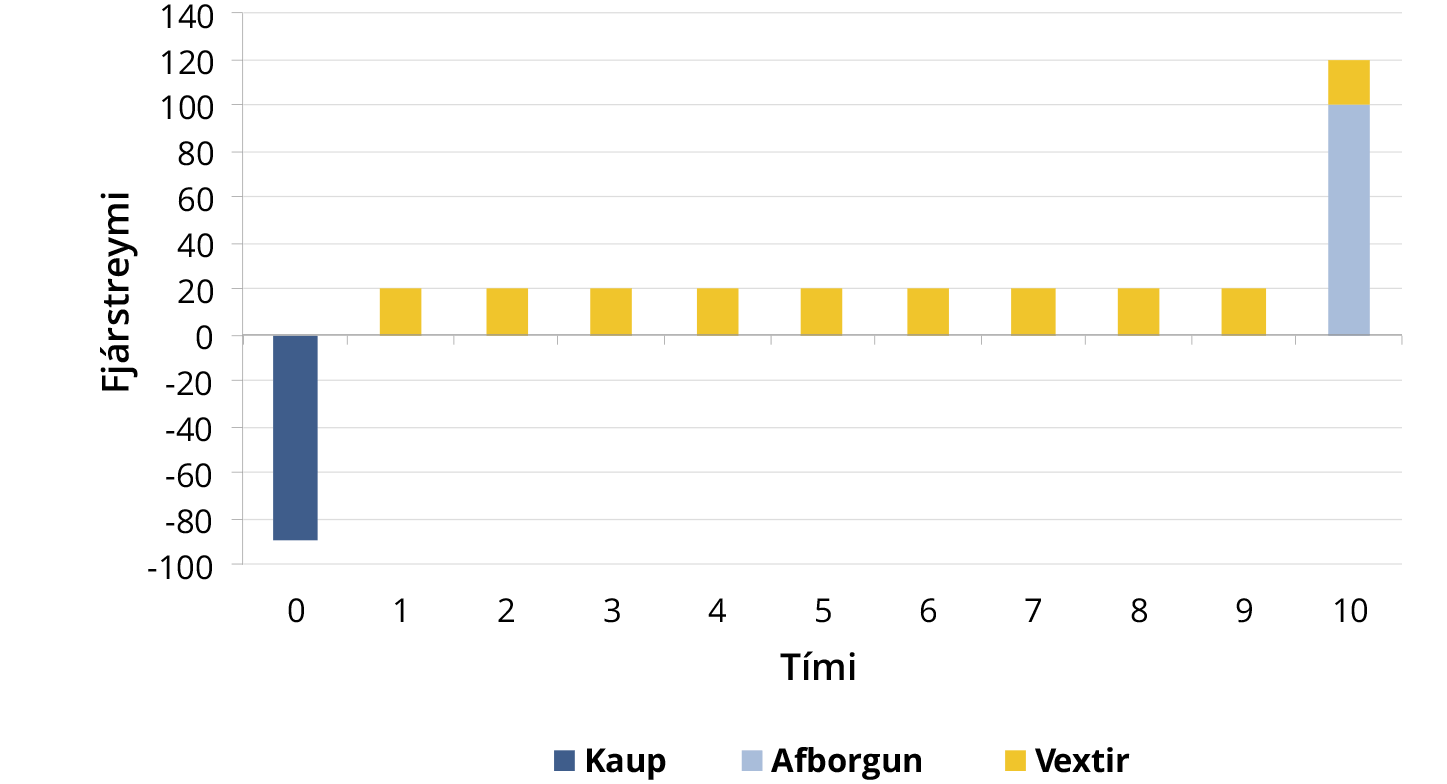
Coupon bond

Interest accrued in each period is paid at the end of that period. No principal is repaid until final maturity.

Example: A 10-year coupon bond with annual payments and 20% nominal interest sold at a price of 90.

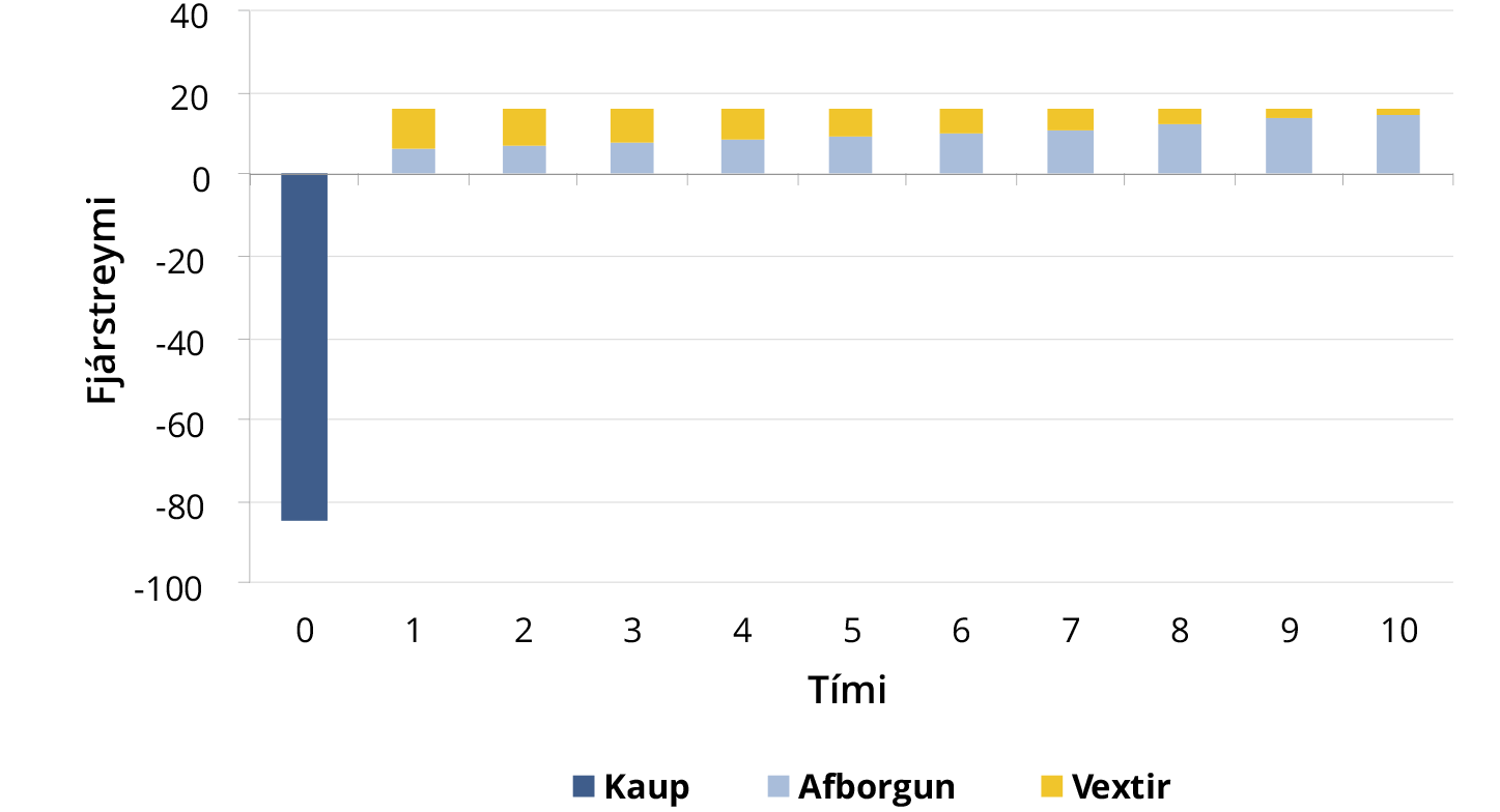
Annuity bond

Every payment on the bond is the same size. Payment = principal repayment + interest accrued in the period.

Example: A 10-year annuity bond with 10% nominal interest sold at a price of 85.

Fixed principal bond

Every repayment of principal is the same size. Interest accrued in each period is paid at the end of that period.

Example: A 10-year fixed principal bond with 12% nominal interest sold at a price of 80.

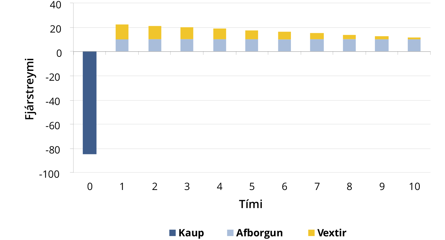
Perpetual bond

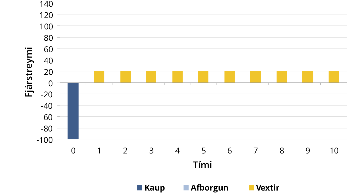
A perpetual bond carries fixed, regular interest payments forever. The principal is never repaid.

Example: A perpetual bond with 20% nominal interest sold at par.

Inflation-indexed bonds

If a bond is non-indexed, its stated rate is the nominal rate, so inflation does not affect its cash flows. If a bond is inflation-indexed, its stated rate is the real rate and both interest and principal payments are linked to the consumer price index, so inflation does affect its cash flows. Indexation ensures that future repayments hold the value they had on the day the loan was made or the saving began.

Bond valuation

The value of a bond is calculated in the same way as the value of a company in equation 1–1: by discounting the expected cash flows back to today at a given required return.

5.1

V_B = \displaystyle\sum_{t=1}^n \frac{INT}{(1+r_d)^t} + \frac{M}{(1+r_d)^n} = INT \cdot (\frac{1 - (1+r_d)^{-n}}{r_d}) + \frac{M}{(1+r_d)^n}

V_B = value of the bond
INT = interest paid on the bond each period
r_d = required return on the bond

M = face value of the bond
n = number of periods

Example 5-1

Áhættusæknir ehf. issues a 15-year coupon bond with annual payments and 10% nominal interest. The face value is ISK 1,000,000 and the required return is 15%. What is the value of the bond?

Solution

In Microsoft ® Excel

Example 5–1 can also be solved with the PV function in Excel:
=PV(rate; nper; pmt; fv)
=PV(15%; 15; -100000; -1000000)
RATE is the required return, NPER the number of periods, PMT the interest payment and FV the face value of the bond.

When the required return on a bond is higher than its nominal rate, as with Áhættusæknir ehf., the bond sells at a discount. When the required return is lower, the bond sells at a premium.

Yield to maturity (YTM)

The return expected on a bond if it is held to final maturity.

Example 5-2

Áhættufælnir ehf. issues a 15-year coupon bond with annual payments and 10% nominal interest. The face value is ISK 1,000,000, but the bond sells for ISK 1,518,983. What is the yield to maturity?

Solution

Unlike the bonds of Áhættusæknir ehf., the required return on the bonds of Áhættufælnir ehf. is lower than the nominal rate, which is why their bonds sell at a premium.

Yield to call (YTC)

A bond with a call provision lets the issuer call the bond and repay the loan before final maturity. If rates fall, the issuer can refinance on better terms, but may in exchange have to pay the bondholder a call premium, most often one year's interest. The yield to call is found by solving for r_d in the following equation:

5.2

V_B = \displaystyle\sum_{t=1}^n \frac{INT}{(1+r_d)^t} + \frac{\text{Call price}}{(1+r_d)^n}

V_B = value of the bond
INT = interest paid on the bond each period
r_d = required return on the bond

M = face value of the bond
n = number of periods
Call price = M + call premium

Example 5-3

Sveigjanlegir ehf. issues a 15-year coupon bond with annual payments and 10% nominal interest. The face value is ISK 1,000,000, but the bond sells for ISK 1,200,000. The bond is callable after 5 years and the call premium is 10% of principal.

a) What is the yield to maturity?b) What is the yield to call?

Solution

Current yield

Defined as the annual interest payment against the current price. Current yield is therefore a measure of a bond's cash flow, but it takes no account of capital gains yield. The total required return on a bond, r_d, as it appears in equation 5-1, is therefore made up of both current yield and capital gains yield.

Credit rating agencies assess the default risk of issuers and assign ratings based on their analysis. The three largest such agencies are (1) Standard & Poor's, (2) Moody's Corporation, and (3) Fitch Group. Their ratings are defined as follows:

Moody's		S&P		Fitch		Description
Long term	Short term	Long term	Short term	Long term	Short term	Description
Aaa	P-1	AAA	A-1+	AAA	F1+	Prime
Aa1		AA+		AA+		High grade
Aa2		AA		AA
Aa3		AA-		AA-
A1		A+	A-1	A+	F1	Upper medium grade
A2		A	A-1	A	F1
A3	P-2	A-	A-2	A	F2
Baa1	P-2	BBB+	A-2	BBB+	F2	Lower medium grade
Baa2	P-3	BBB	A-3	BBB	F3
Baa3	P-3	BBB-	A-3	BBB	F3
Ba1	Not prime	BB+	B	BB+	B	Non-investment grade / speculative / junk
Ba2		BB		BB
Ba3		BB-		BB-
B1		B+		B+		Highly speculative
B2		B		B
		B3		B-
Caa1		CCC+	C	CCC	C	Substantial risks
Caa2		CCC				Extremely speculative
Caa3		CCC				In default with little prospect for recovery
Ca		CC
Ca		C
C		D	/	DDD	/	In default
/				DD
/				DD

The annual accounts

A company's balance sheet is often shown graphically as in figure 6–1, which sets out how assets = liabilities + equity, and how assets divide into current assets and fixed assets, and liabilities into current liabilities and long-term liabilities.

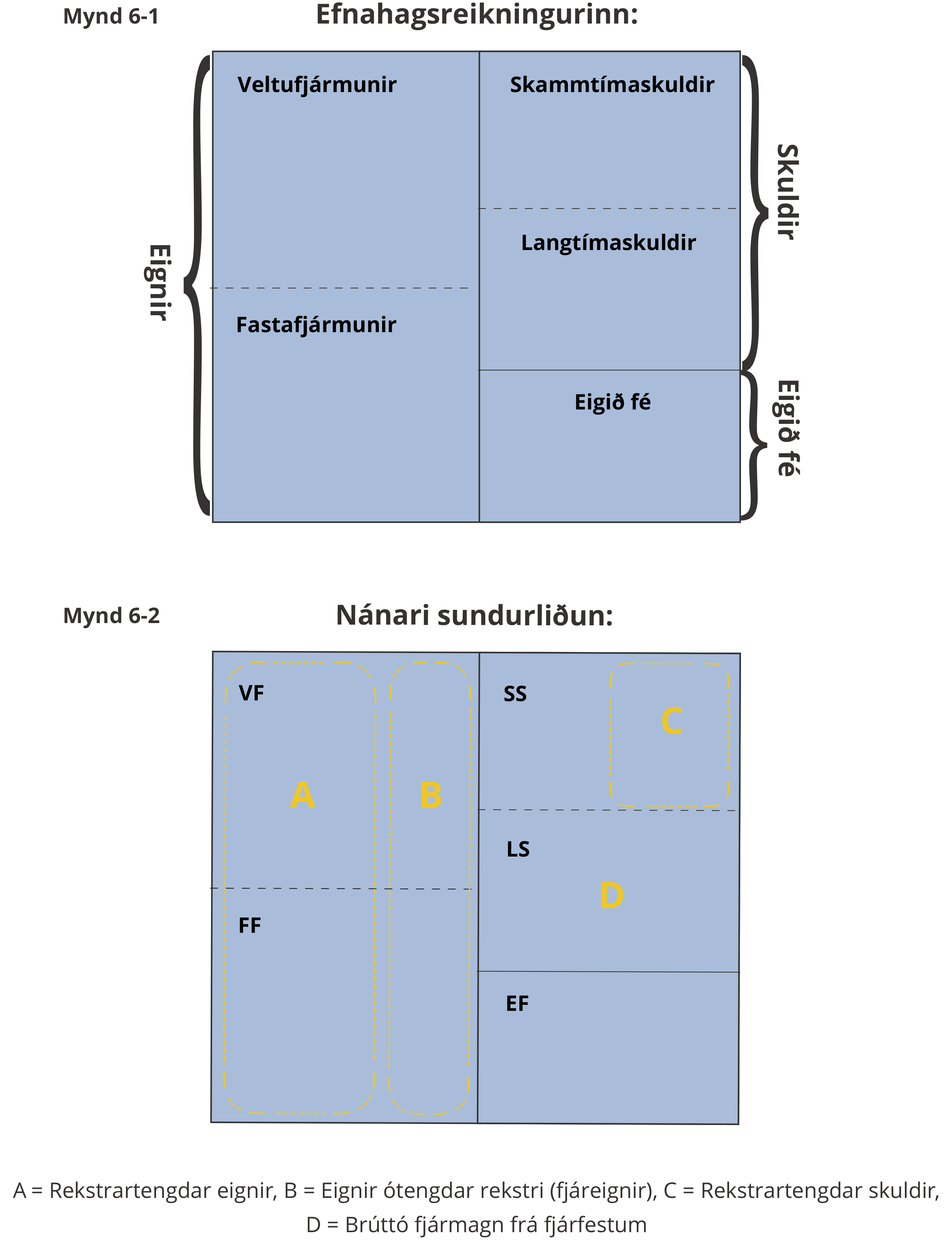
To find operating capital (OC), the balance sheet is split up as in figure 6–2, where A+B = C+D and therefore also A–C = D–B.

6.1

Operating capital (OC) =A - C = Operating assets - Operating liabilities

6.2

Net capital from investors =D - B = Gross capital from investors - Non-operating assets

Net operating profit after taxes (NOPAT) is the profit a company would report if it had no debt and held no financial assets.

6.3

Net operating profit after taxes (NOPAT) =EBIT·(1-tax rate)

EBIT = earnings before interest and taxes

The cash flow available to all investors after a company has invested enough in operating capital (OC) to sustain continuing operations is called free cash flow (FCF).

6.4

Free cash flow (FCF) =NOPAT - net investment in OC = NOPAT - gross investment in OC + depreciation

To see how well a company uses its operating capital to generate profit, look at return on invested capital (ROIC).

6.5

Return on invested capital (ROIC) =

\frac{NOPAT}{OC}

One of the most common measures in value-based management is economic value added (EVA), which measures the effect of investment, cost of capital and operations on the value of a company.

6.6

Economic value added (EVA) =

NOPAT - (OC \cdot WACC) = OC \cdot (ROIC-WACC)

The weighted average cost of capital (WACC) is covered in more detail in part 8, but equation 6–6 shows that a company only increases its value if ROIC > WACC.

Financial ratios

Financial ratios are grouped here into five categories: (1) profitability, (2) liquidity, or a company's ability to pay its debts, (3) coverage ratios, or a company's financial strength and room to grow, (4) activity ratios, and (5) market value.

Profitability ratios

7.1

Return on equity (ROE) =Profit/Average equity

7.2

Return on assets (ROA) =Profit/Average total assets

7.3

Profit margin =Profit/Sales

7.4

Gross profit margin =Gross profit/Sales

7.5

Payout ratio =Dividends/Profit

Liquidity ratios

7.6

Current ratio =Current assets/Current liabilities

7.7

Quick ratio (acid test) =Quick assets/Current liabilities

Quick assets = Current assets - Inventory

7.8

Cash ratio =(Cash + short-term securities)/Current liabilities

7.9

Current cash debt coverage ratio =Cash flow from operations/Average current liabilities

7.10

Quality of earnings =Cash flow from operations/Profit

Coverage ratios

7.11

Debt to assets ratio =Total liabilities/Total assets

7.12

Equity ratio =Equity/Total assets

7.13

Times interest earned (TIE) =(Operating profit (EBIT))/Interest expense

7.14

Cash debt coverage ratio =Cash flow from operations/Average total liabilities

Activity ratios

7.15

Asset turnover ratio =Operating revenue/Average total assets

7.16

Inventory turnover ratio =Cost of goods sold/Average inventory

7.17

Receivables turnover ratio =(Total sales - Cash sales)/Average trade receivables

7.18

Accounts payable turnover =Cost of goods sold/Average trade payables

Market value ratios

7.19

Price/earnings ratio (P/E ratio) =Market price per share/Earnings per share

7.20

Market/book ratio =Market capitalisation/Equity

7.21

Book value per share (BVPS) =Ordinary shareholders' equity/Number of ordinary shares outstanding

7.22

Dividend yield =Dividend/Market price

7.23

Earnings per share (EPS) =Profit/Average shares outstanding

7.24

Internal value of shares =Equity/Share capital

7.25

Price/earnings to growth ratio (PEG ratio) =(P/E ratio)/Earnings growth in %

Cost of capital

The weighted average cost of capital (WACC) is the average cost to a company of raising the capital it uses to fund its operations.

8.1

Weighted average cost of capital (WACC) =

w_d r_d (1-T) + w_{ps} r_{ps} + w_{ce} r_s

w_d, w_ps and w_ce = weights for debt (d), preferred stock (ps) and common equity (ce), so that w_d + w_ps + w_ce = 1
r_d = required return on debt
T = tax rate

r_ps = required return on preferred stock
r_s = required return on common equity

There are various ways to calculate r_s; two are given here. The first is to use the capital asset pricing model (CAPM) and apply the security market line (SML) equation (see equation 4–2):

8.2

r_s = r_{RF} + (r_M - r_{RF}) \cdot b_s = r_{RF} + (RP_M) \cdot b_s

r_s = required return on share s
r_M = required return on the market portfolio
r_RF = risk-free rate of return on treasury bills

RPM = r_M - r_RF = the market risk premium
b_s = beta of share s
(r_M - r_RF · b_s = risk premium on share s

The second is to use the Gordon growth model and apply the following equation:

8.3

r_s = \frac{D_0 \cdot (1+g)}{P_0} + g = \frac{D_1}{P_0} + g

D₀ = the most recent dividend
D₁ = expected dividend one year from now
P₀ = price of share s today
g = expected dividend growth

Example 8-1

Shares in Stórfyrirtæki hf. are valued at ISK 30 per share, and the company paid a dividend of ISK 3 per share last year. Expected dividend growth is 5%.
What is the required return on shares in Stórfyrirtæki hf.?

Solution

Equity can be raised by retaining earnings from previous years or by issuing new shares on the stock market. The latter carries a flotation cost (F), which must be taken into account when calculating r_s.

8.4

r_e = \frac{D_1}{P_0 (1-F)} + g

r_e = required return on external equity (e)
D₁ = expected dividend one year from now
P₀ = price of share s today

F = flotation cost
g = expected dividend growth

Company valuation

As figure 6–2 shows, a company's assets split into A, operating assets and B, non-operating assets. The value of operations (V_op) is the sum of all free cash flow (FCF) from the operating assets, discounted at the weighted average cost of capital (WACC).

9.1

V_{op} = \displaystyle\sum_{t=1}^\infty \frac{FCF_t}{(1+WACC)^t} = \frac{FCF_1}{(1+WACC)^1} + \frac{FCF_2}{(1+WACC)^2} + \cdots + \frac{FCF_\infty}{(1+WACC)^\infty}

D₀ = the most recent dividend
D₁ = expected dividend one year from now
P₀ = price of share s today
g = expected dividend growth

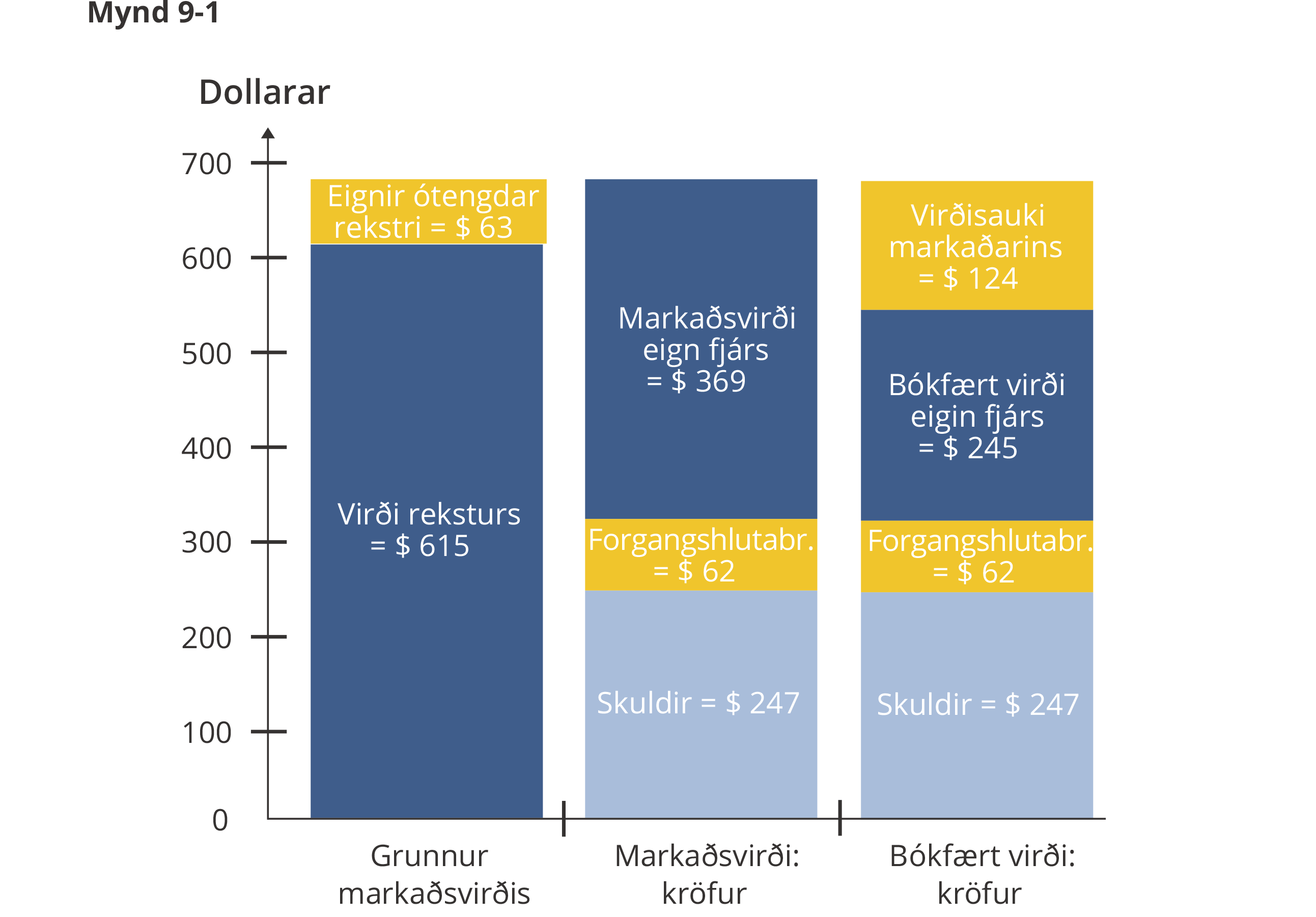
The total value of the company is shown in figure 9–1 and is made up of the value of operations, V_op, plus the value of non-operating assets.

9.2

Total value of company =V_op + value of non-operating assets

The market value of equity is then the total value of the company less the value of debt and preferred stock.

9.3

Market value of equity =Total value of company - Value of debt and preferred stock

The book value of equity can be read from the company's annual accounts, but it can also be described like this:

9.4

Book value of equity =Market value of equity - Market value added (MVA)